Eigen Value Decomposition

Overview

Eigen Value Decomposition (EVD) is one of the most fundamental matrix factorizations in linear algebra. While EVD is only applicable to square matrices, it lays the foundation for SVD which is applicable to any matrix. Here, we will explore the relationship between SVD and EVD.

Mathematical Foundations

Definition

For a square matrix \(A \in \mathbb{R}^{n \times n}\), eigendecomposition is:

\[A = Q \Lambda Q^{-1}\]

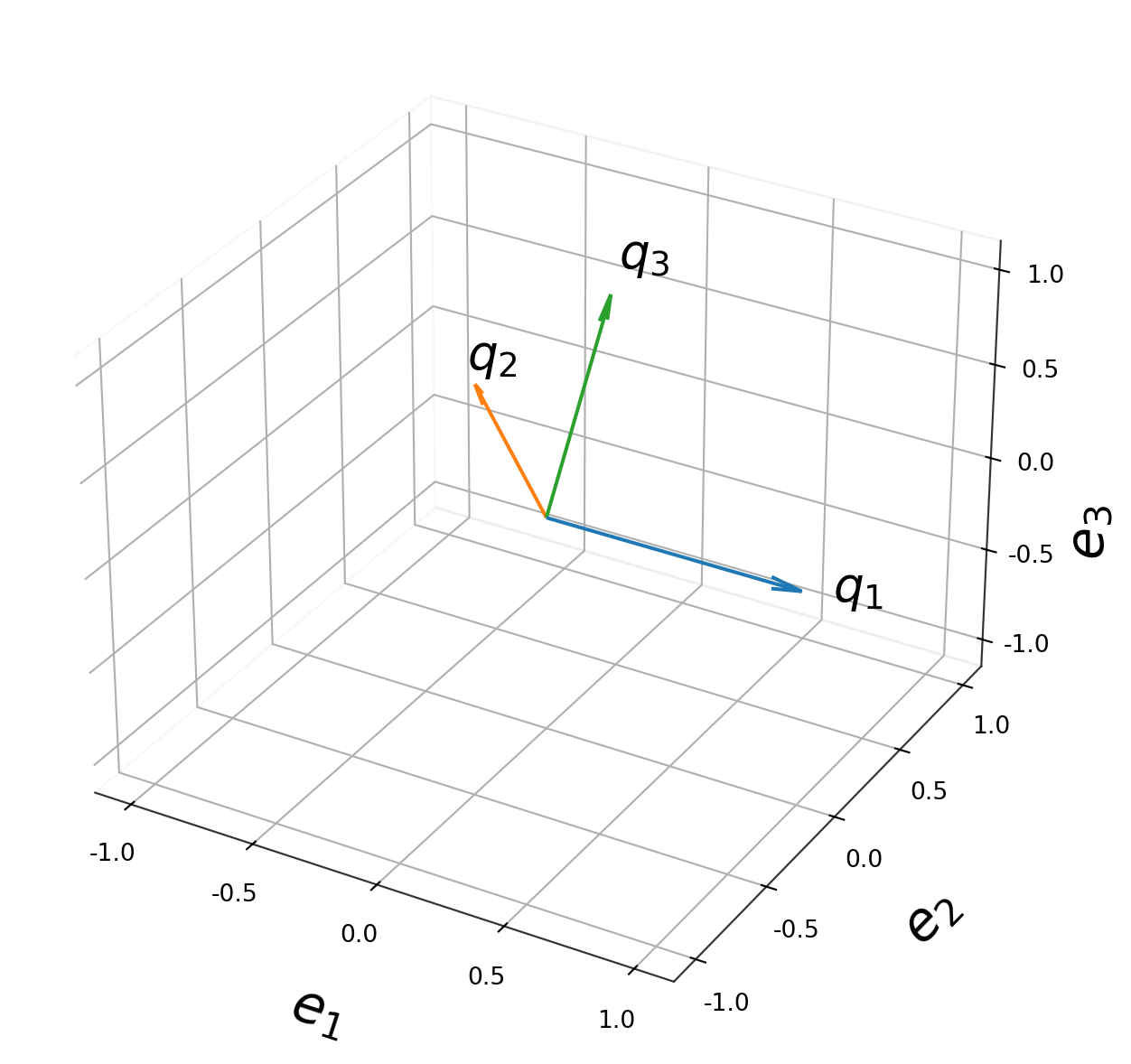
where: - \(Q \in \mathbb{R}^{n \times n}\) — matrix of eigenvectors as columns - \(\Lambda = \text{diag}(\lambda_1, \lambda_2, \dots, \lambda_n)\) — diagonal matrix of eigenvalues (can be complex!)

The core relationship is:

\[A q_i = \lambda_i q_i\]

For symmetric matrices (\(A = A^T\)), this simplifies to:

\[A = Q \Lambda Q^T \qquad \text{(spectral theorem)}\]

since eigenvectors of symmetric matrices are orthogonal.

Outer Product (Sum) Form

EVD can be written as a sum of outer products of eigenvectors and eigenvalues:

\[A = \sum_{i=1}^{n} \lambda_i \, q_i \, p_i^T\]

where \(q_i\) is the \(i\)-th eigenvector and \(\lambda_i\) is the \(i\)-th eigenvalue and \(p_i\) is the \(i\)-th eigenvector of \(A^T\), and \(p_i\) is the \(i\)-th column on \(Q^{-1}\).

If \(A\) is symmetric, then \(p_i = q_i\), and the formula simplifies to:

\[A = \sum_{i=1}^{n} \lambda_i \, q_i \, q_i^T\]

Spectral Theorem

The spectral theorem states that any symmetric matrix can be written as a sum of outer products of eigenvectors and eigenvalues:

\[A = Q \Lambda Q^T\]

SVD vs. EVD

Key Differences

Property	SVD	EVD
Applicable to	Any \(m \times n\) matrix	Square \(n \times n\) matrices only
Factorization	\(A = U\Sigma V^T\)	\(A = Q\Lambda Q^{-1}\)
Two vector spaces	Left (\(U\)) and right (\(V\)) are different	Same vector space for input and output
Values on diagonal	\(\sigma_i \geq 0\) always real, non-negative	\(\lambda_i \in \mathbb{C}\) can be complex
Factor matrices	\(U, V\) always orthogonal	\(Q\) orthogonal only if \(A\) is symmetric
Uniqueness	Always exists	May not exist (defective matrices)
Geometry	Rotation → stretch → rotation	Stretch along eigenvectors

The Deep Connection

For a symmetric positive semidefinite matrix \(A = A^T \geq 0\), SVD and EVD coincide:

\[A = Q\Lambda Q^T = U\Sigma V^T \quad \Rightarrow \quad U = V = Q, \quad \Sigma = \Lambda\]

For a general square matrix \(A\), SVD works on \(A^T A\) and \(AA^T\):

\[A^T A = V \Sigma^T \Sigma V^T \quad \text{(eigendecomposition of } A^T A\text{)}\] \[A A^T = U \Sigma \Sigma^T U^T \quad \text{(eigendecomposition of } A A^T\text{)}\]

So singular values of \(A\) are the square roots of eigenvalues of \(A^T A\):

\[\sigma_i(A) = \sqrt{\lambda_i(A^T A)}\]

When is \(Q^{-1} = Q^T\)?

\(Q^{-1} = Q^T\) holds if and only if \(Q\) is an orthogonal matrix, meaning its columns are orthonormal. This only happens when \(A\) is a normal matrix, defined by:

\[A A^T = A^T A\]

So the correct general form always requires the full inverse:

\[A = Q \Lambda Q^{-1}\]

and simplifies to \(Q\Lambda Q^T\) only under the special condition \(AA^T = A^TA\). This is precisely what makes SVD more powerful — it always uses orthogonal matrices \(U\) and \(V\) with \(U^{-1} = U^T\) and \(V^{-1} = V^T\), at the cost of needing two different orthogonal bases instead of one.

Finding Eigenvalues and Eigenvectors

Step 1: What We Need to Solve

We want to find all scalars \(\lambda\) and non-zero vectors \(q\) such that:

\[Aq = \lambda q\]

The key constraint is \(q \neq 0\) — a zero vector is a trivial, useless solution.

Step 2: Rearrange Into a Homogeneous System

Rewrite the equation by moving everything to one side:

\[Aq - \lambda q = 0\]

\[Aq - \lambda I q = 0\]

\[\underbrace{(A - \lambda I)}_{\text{some matrix}} q = 0\]

So we need a non-zero vector \(q\) that gets mapped to zero by the matrix \((A - \lambda I)\). This is asking: does \((A - \lambda I)\) have a non-trivial null space?

Step 3: The Critical Insight: When Does a Non-Zero Solution Exist?

For the system \(Mq = 0\), recall from linear algebra:

\[Mq = 0 \text{ has a non-zero solution} \iff M \text{ is singular} \iff \det(M) = 0\]

This is because: - If \(M\) is invertible, the only solution is \(q = M^{-1} \cdot 0 = 0\) — useless - If \(M\) is singular, it collapses space, and some non-zero vector gets mapped to zero — exactly what we want

So the condition becomes:

\[\det(A - \lambda I) = 0\]

This is the characteristic equation, and it is the entire reason the determinant appears.

Step 4: The Characteristic Polynomial

Expanding \(\det(A - \lambda I)\) gives a polynomial in \(\lambda\) of degree \(n\):

\[p(\lambda) = \det(A - \lambda I) = (-1)^n \lambda^n + c_{n-1}\lambda^{n-1} + \cdots + c_1 \lambda + c_0 = 0\]

For a \(2 \times 2\) matrix \(A = \begin{pmatrix} a & b \\ c & d \end{pmatrix}\):

\[A - \lambda I = \begin{pmatrix} a - \lambda & b \\ c & d - \lambda \end{pmatrix}\]

\[\det(A - \lambda I) = (a-\lambda)(d-\lambda) - bc = 0\]

\[\lambda^2 - \underbrace{(a+d)}_{\text{trace}} \lambda + \underbrace{(ad - bc)}_{\det(A)} = 0\]

Notice the beautiful identities baked in:

\[\lambda_1 + \lambda_2 = \text{tr}(A) = a + d\]

\[\lambda_1 \cdot \lambda_2 = \det(A) = ad - bc\]

Step 5: Find eigenvalues: solve \(\det(A - \lambda I) = 0\)

\[\det(A - \lambda I) = 0 \quad \Rightarrow \quad \lambda_1, \lambda_2, \dots, \lambda_n\]

Step 6: Find eigenvectors: for each \(\lambda_i\), solve \((A - \lambda_i I)q = 0\)

This is just Gaussian elimination (row reduction) on the matrix \((A - \lambda_i I)\).

Worked Example

Let \(A = \begin{pmatrix} 3 & 1 \\ 0 & 2 \end{pmatrix}\)

Step 1: Characteristic equation

\[\det(A - \lambda I) = \det\begin{pmatrix} 3-\lambda & 1 \\ 0 & 2-\lambda \end{pmatrix} = (3-\lambda)(2-\lambda) - 0 = 0\]

\[\lambda^2 - 5\lambda + 6 = 0 \implies (\lambda - 3)(\lambda - 2) = 0\]

\[\boxed{\lambda_1 = 3, \quad \lambda_2 = 2}\]

Step 2a: Eigenvector for \(\lambda_1 = 3\)

\[(A - 3I)v = \begin{pmatrix} 0 & 1 \\ 0 & -1 \end{pmatrix} \begin{pmatrix} v_1 \\ v_2 \end{pmatrix} = \begin{pmatrix} 0 \\ 0 \end{pmatrix}\]

Both rows say \(v_2 = 0\), and \(v_1\) is free:

\[\boxed{v^{(1)} = \begin{pmatrix} 1 \\ 0 \end{pmatrix}}\]

Step 2b: Eigenvector for \(\lambda_2 = 2\)

\[(A - 2I)v = \begin{pmatrix} 1 & 1 \\ 0 & 0 \end{pmatrix} \begin{pmatrix} v_1 \\ v_2 \end{pmatrix} = \begin{pmatrix} 0 \\ 0 \end{pmatrix}\]

One equation: \(v_1 + v_2 = 0 \implies v_1 = -v_2\), with \(v_2\) free:

\[\boxed{v^{(2)} = \begin{pmatrix} -1 \\ 1 \end{pmatrix}}\]